


Academic epidemiology & research
Rigorous spatial methods without writing the pipeline.
Run Local Cluster Analysis and geographically weighted regression on public county data, then share a read-only project with co-authors (they need Vesta accounts) or export the results and a report for the manuscript.
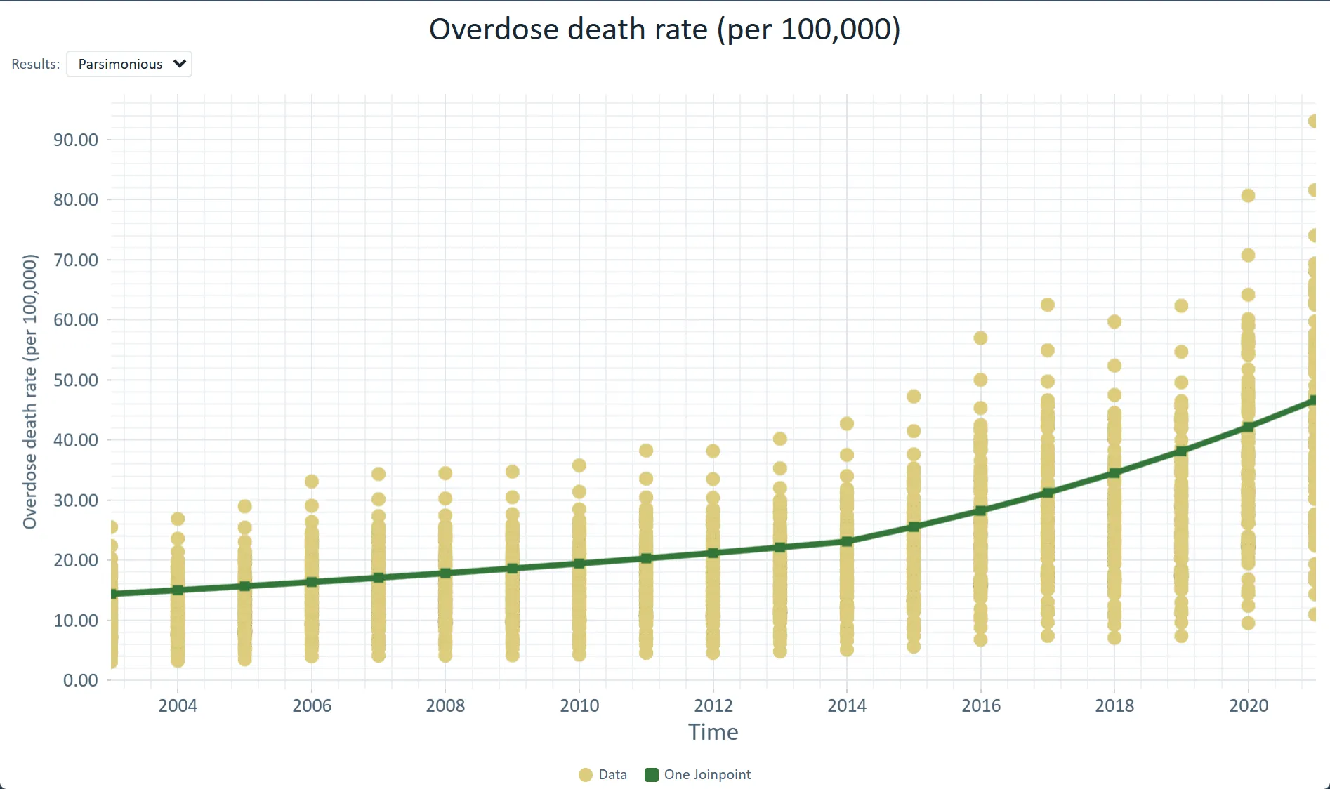
 County overdose death rates with the statewide joinpoint trend (2014) · Ohio, 2003–2021
The challenge
Building a spatial pipeline in R or Python takes weeks, and hand-off to students or co-authors is fragile.
Step 1Share one projectShare the project by email: Can view for co-authors who only read it, Can duplicate for those who want their own copy. An address without a Vesta account gets a read-only link instead.How to: Sharing projects
Step 2Find the clustersLocal Cluster Analysis flags High-High and Low-Low counties, with an optional false discovery rate correction and a seed so the run can be repeated.How to: Local cluster analysis
Step 3Model the relationshipGeographically weighted regression shows how a predictor's effect changes across the map; read the local R-squared and the residual Moran's I.How to: Regression and GWR
Step 4PublishExport the results and a report as supplementary material for the manuscript.How to: Exporting data and pictures
Worked example · Diabetes and poverty
How much of the county variation in diagnosed diabetes does poverty explain, and where do high rates cluster?
- Start from the counties3,109 counties with diagnosed diabetes (CDC PLACES, 2024 release) and poverty (ACS 2022), on one county layer.How to: Data Library
- Test the clustersLocal Moran's I with queen contiguity, 999 permutations, a false discovery rate of 0.05 and seed 2026: global I is 0.625, with 357 High-High counties and 389 Low-Low.How to: Local cluster analysis
- Fit the poverty effectGWR of diabetes on poverty: global R-squared 0.753, local R-squared from 0.06 to 0.96, and a residual Moran's I of 0.009.How to: Regression and GWR
What it found
Diabetes clusters across the South (357 High-High counties), with 389 Low-Low counties. The local poverty slope runs from about −0.35 to 0.66 points of diabetes per point of poverty, steepest across much of the Southeast.
Both variables are estimates, not counts: PLACES is model-based and the ACS is a sample survey. The clusters show where groups sit, not why.
Local Moran's I clusters · diabetes among U.S. adults, by county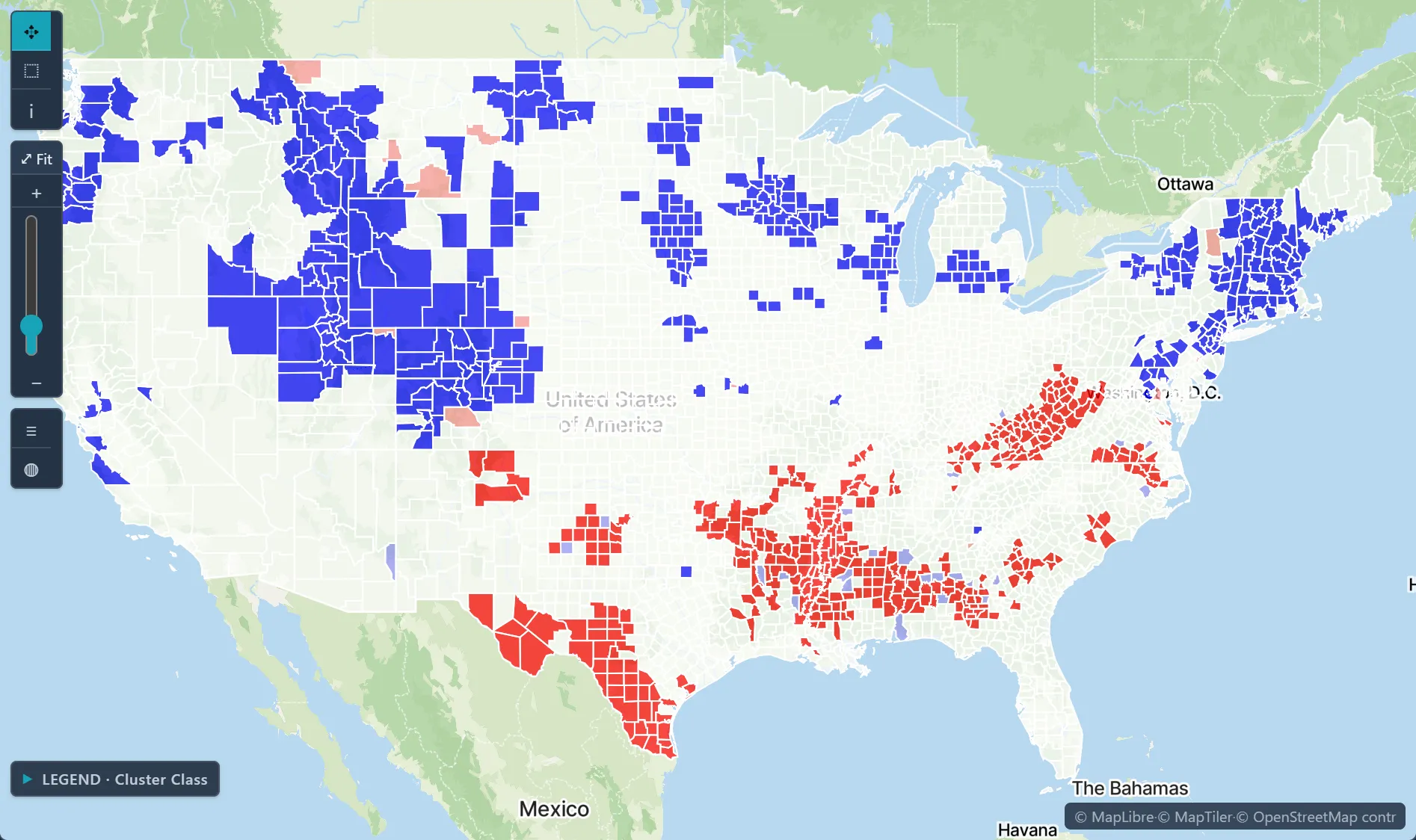
Open the sample projectRead-only · no sign-in
Read in the docs
Methods
Local Cluster AnalysisRegression and GWRJoinpoint regressionScan statisticsKriging
Data
Your study dataCDC PLACESACS 5-Year Data Profiles
Evidence
Published research by BioMedware scientistsLocal bladder cancer clusters in southeastern Michigan accounting for risk factors, covariates and residential mobilityJacquez, G.M., Shi, C., Meliker, J.R. PLOS ONE 10, 2015.
See every sample project